Invalid data dump - Amazon Redshift, Data Pipeline and S3

Amazon Data Pipeline (DPL) is late entrant to the ETL market but provides many features that are well integrated to AWS cloud.  In any data extraction process one would encounter invalid or incorrect data and that data may either be logged or ignored depending on the business requirements or severity of rejected data.

When you have your data flow through S3 to other platforms, be it, Redshift, RDS, DynamoDB, etc. in AWS you can use S3 to dump that data.   In an example, similar to one DPL below, in one of the step you could filter and dump to S3 for later analysis.


By standardizing the rejections from different DPLs, another DPL can regularly load them back into Redshift for quick realtime analysis or deep dive into them downstream.  This will also greatly help in recovery and reruns when needed.

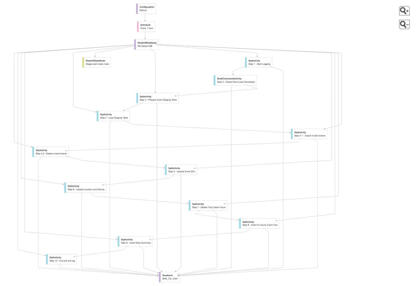
Following is simple high level steps where rejected data is directed to S3.  The parameters are provided through the environment setup.  For example: #{myDPL_schema_name} = 'prod_public' and #{myDPL_error_log_path} = 's3://emr_cluster/ad/clicks/...'


-- PreProcess 
-- Load staging stable and at the same time update data error column in it when possible.
INSERT INTO #{myDPL_schema_name}.#{myDPL_staging_table}
SELECT col1,
  col2,
  col3,
  etc
  CASE WHEN 
  AS data_error
FROM #{myDPL_schema_name}.#{myDPL_source_table}
LEFT OUTER JOIN #{myDPL_schema_name}.table_1
  ON ...
LEFT OUTER JOIN #{myDPL_schema_name}.dim_1
  ON ... 
LEFT OUTER JOIN #{myDPL_schema_name}.dim_N
  ON ...
WHERE ...


-- OR, If data_error column is updated separately...
UPDATE #{myDPL_schema_name}.{myDPL_staging_table}
SET data_error = ...
FROM #{myDPL_schema_name}.{myDPL_staging_table}
JOIN #{myDPL_schema_name}.dim_1
JOIN #{myDPL_schema_name}.dim_N
WHERE ...

-- Temporary table
CREATE TEMP TABLE this_subject_dpl_rejections AS (
SELECT
  ...
FROM #{myDPL_schema_name}.#{myDPL_staging_table}
WHERE data_error IS NOT NULL
);

-- Dump to S3
UNLOAD ('SELECT * FROM this_subject_dpl_rejections')
TO '#{myDPL_ErrorLogPath}/yyyy=#{format(@scheduledStartTime,'YYYY')}/
  mm=#{format(@scheduledStartTime,'MM')}/dd=#{format(@scheduledStartTime,'dd')}/
  hh=#{format(@scheduledStartTime,'HH')}/ran_on_#{@actualStartTime}_file_'
CREDENTIALS 'aws_access_key_id=#{myDPL_AWSAccessKey};aws_secret_access_key=#{myDPL_AWSSecretKey}'
GZIP
PARALLEL OFF
ALLOWOVERWRITE;
Now load the errors back to Redshift...
COPY #{myDPL_schema_name}.#{myDPL_error_table}
FROM  '#{myDPL_ErrorLogPath}/yyyy=#{format(@scheduledStartTime,'YYYY')}/
  mm=#{format(@scheduledStartTime,'MM')}/dd=#{format(@scheduledStartTime,'dd')}/ 
  hh=#{format(@scheduledStartTime,'HH')}/'
CREDENTIALS 'aws_access_key_id=#{myDPL_AWSAccessKey};aws_secret_access_key=#{myDPL_AWSSecretKey}'
DELIMITER  '|' 
GZIP 
TRIMBLANKS
TRUNCATECLUNS 
IGNOREBLANKLINES

Amazon CloudTrail parsing for specific API call using Spark

Recently I needed to parse Amazon Web Service CloudTrail log files to check for some specific API call.  The call was being deprecated by Amazon and we needed to upgrade our code to reflect the latest CLI (aws).  The logs I got from IT folks were json files and each file contained only one single line each with length anywhere from 0.5MB to 1MB! And this one line had array of json objects like below.

Problem:  Identify an application that is making some specific API calls to a service.   Not much other info was available and all we had was bunch of CloudTrail logs and AWS deprecated API call (DescribeJobFlows).
See - http://docs.aws.amazon.com/ElasticMapReduce/latest/API/API_DescribeJobFlows.html which basically suggested "DescribeJobFlows: This API is deprecated and will eventually be removed. We recommend you use..."

{"Records": [ {"eventVersion":"1.02","userIdentity":{"type":"IAMUser","principalId":"AIDAIVWSMF.........","arn":"arn:aws:iam::144..........:user/staging-user","accountId":"14    4702935796","accessKeyId":".............","userName":"............."},"eventTime":"2016-.....T13:50:16Z","eventSource":"datapipeline.amazonaws.com","eventName":"Report    TaskProgress","awsRegion":"us-east-1","sourceIPAddress":"54.2.......","userAgent":"aws-sdk-java/unknown-version Linux/3.4.73-64.112.amzn1.x86_64 OpenJDK_64-Bit_Server_VM/23    .25-b01/1.6.0_33","requestParameters":{"taskId":"37kSdZbBpwRjSng--/1Tms+pYiDGRURfXkPWl90Azl893QqHry1pryPTkUzLed5u1O2KIK9qh8pM1fk8fPBHzGbHDWhk0VTWFru3wJnanhJSuYLkEZ0fSmC...."},"responseElements":{"canceled":false},"requestID":"65ac3d1a-476e-11e6-a25c-f339ebc3012a","eventID":"4b4ebf63-0fd3-4f1e-81c0-0b399dd07a69","eventType":"AwsApiC    all","recipientAccountId":"144........"},....

It is actually array of JSON objects and for more info on the log see http://docs.aws.amazon.com/awscloudtrail/latest/userguide/view-cloudtrail-events-cli.html

Even before developing some code I wanted to test couple of ideas.  Following is one of the way I was able to identify the offending application and host(s).  After the successful evaluation, I wrote Python script to upload hundreds of files to S3's new bucket and performed minor transformation to clean the data so that data was suitable for loading to Spark.

For quick readable json you can do:

> vim 144........._CloudTrail_us-east-1_20160711T1355Z_n0m854FRPqpkaPd3.json
 # and then using python json module
(in vim) :%!python -m json.tool
to see
    1  {                                                                                                                                                                          
    2     "Records": [
    3         {
    4             "awsRegion": "us-east-1",
    5             "eventID": "4b4ebf63-0fd3-4f1e-81c0-0b399dd07a69",
    6             "eventName": "ReportTaskProgress",
    7             "eventSource": "datapipeline.amazonaws.com",
    8             "eventTime": "2016-.....T13:50:16Z",
    9             "eventType": "AwsApiCall",
   10             "eventVersion": "1.02",
   11             "recipientAccountId": "144...",
   12             "requestID": "65ac3d1a-476e-11e6-a25c-f339ebc3012a",
   13             "requestParameters": {
   14                 "taskId": "37kSdZbBpwRjSng/1Tms+p....
   16             "responseElements": {
   17                 "canceled": false
   18             },
   19             "sourceIPAddress": "54........",
   20             "userAgent": "aws-sdk-java/unknown-version Linux/3.4.73-64.112.amzn1.x86_64 OpenJDK_64-Bit_Server_VM/23.25-b01/1.6.0_33",
   21             "userIdentity": {
   22                 "accessKeyId": "AK...",
   23                 "accountId": "144...",
   24                 "arn": "arn:aws:iam::144....:user/staging-user",
   25                 "principalId": "...",
   26                 "type": "IAMUser",
   27                 "userName": "....-user"
   28             }
   29         },
   30         {
 
will spit out readable output.   Next is performing some cleanup and have one json object per line.

(in vim) :1,$s#\{\"Records\"\:\ \[##     -- vim removal of header
(in vim) :1,$s#\}\,#\}^V^M#g               -- vim substitute each record onto it's own line

I then loaded his file into Spark table and then run SparkSQL on it.   See screenshots below.


Note "DescribeJobFLows" calls above originating from an EMR instance on a specific IP.

Simple puzzle and memory usage

Recently there was a simple puzzle in one of my whatsapp group.  It was
if 1 => 8, 2 =>  18,
   3 =>  30, 4 =>  44, 5 =>  60, then what is 9?

It was simple to calculate by hand and provide the answer.  You can also formulate the above deduction and use it for any number with

6 + (M + (2 x n))
    where n is set of integers; 0 < n < N
    and M is cumulative sum from previous step with M(initial value) is 0

This problem lends itself well to reduction function and with the given formula it was easy to check it for any integer n.  Out of curiosity created a function and was called in Python for-loop for each iteration while monitoring load on CPU and memory tracked. Then I used reduce function with xrange to see the same.

# Python

>>> a = []; M = 0

>>> for n in range(0, 100000000):
...        M = 6+M+(2*n)
...        a.append(M)

# [ CPU was loaded above 97% with memory usage jumping and ended up killing the process ]


>>> print reduce(lambda x,y: 6+x+(2*y), xrange(0,100000000))

10000000499999994

# with xrange, got the result in less than few seconds though CPU usage jumped above 97% but no discernible change in memory.   

Visualizing data processed consciously in a moment

Recently Google released a training material to its employees as part of how unconscious bias can happen in work place.  For more details see -
http://www.businessinsider.com/google-unconscious-bias-training-presentation-2015-12  which refers to research paper at http://rd.springer.com/chapter/10.1007%2F978-3-642-82598-9_3

It is very interesting and one of the slide (see below) specifically caught my attention with respect how huge amount of data is NOT processed consciously.   That is we can only handle 40 bits for every 11 million bits in a second!

That is just 1 part for every 275,000 parts!!


As interesting as it is the impact I thought will be even more dramatic when visualized it in some way.  Following are of couple of attempts at it using Python and ImageMagick.

Each tiny square (green or red) in the following picture represents 40 bits and each row has 275 of those squares. With 1000 rows (10 blocks of 100 rows each) of those we get 11 Million bits of data represented.  This is just for one second of duration!


Just imagine the the scale for one's life time (80 years) data. All those 275,000 blocks above are to be repeated 2,522,880,000 times!!!


Another way is tiny string, say 5 pixels long, represents 40 bits then total length of 11M bits will be 275k * 5 pixels long!  See below.  Small green line at the center of the diagram is a string of few pixels and around which the really long string i.e., 275K times long string is wound around a square peg. At each of 25 rounds the string changes color for better visibility. Totally there are 742 sides.

at end of 25th round the length is 5,050 times longer and
at end of 50th round it is 20,100 times
at end of 100th round it is 80,200 times
at end of 150th round it is 180,300 times
and finally at 185.25 round it is 274,111 times longer

Note: Keep in mind it is not the size (area) of the squares but the total perimeter length of all these squares that represents ratio of data.

Check and set analyze statistics on tables-columns in Vertica

It is important to update statistics in any database for better query runs or query optimizations.  Vertica provides ANALYZE_STATISTICS and ANALYZE_HISTOGRAM to collect stats and in big data warehouse environment it is sometime possible that some tables may not have stats collected.  In that case you can run following query to check and add the tables/ columns to collect stats.


SELECT T1.table_schema, T1.table_name, T2.row_ct, T2.wos_ct, T2.ros_ct FROM ( -- Get list of tables that don't have 'FULL' stats SELECT distinct table_schema, table_name FROM projection_columns WHERE (statistics_type = 'ROWCOUNT' or statistics_type = 'NONE') -- and table_schema not like 'v_%' AND (table_schema = 'schema_1' OR table_schema = 'schema_2' ) ORDER BY 1,2 ) T1 JOIN ( -- Get list of tables with storage details SELECT anchor_table_schema, anchor_table_name, sum(row_count) row_ct, sum(wos_row_count) wos_ct, sum(ros_row_count) ros_ct FROM projection_storage WHERE (anchor_table_schema = 'schema_1' OR anchor_table_schema = 'schema_2' ) GROUP BY 1,2 ) T2 ON T1.table_schema = T2.anchor_table_schema AND T1.table_name = T2.anchor_table_name ORDER BY 3 desc;

From the list generated above add those tables/ columns to your regular stats collecting script which you can run during off peak hours.

Notes:
Vertica's ANALYZE_HISTOGRAM returns similar data as ANALYZE_STATISTICS except that one can set the percent of data that is sampled to generate statistics metrics.  In the case of latter it uses fixed 10% sampling.

WOS: Write Optimized Store is a memory resident data structure used to support fast data loads without data compression and indexing.
ROS: Read Optimized Store is disk-based storage with data compressed and sorted.  Tuple Mover moves data out of WOS and into ROS in batches.

References:

Removing duplicates in Vertica data sets

Many a time due to bug or otherwise duplicate rows gets introduced into tables and it is not hard to perform dedupe and let the ETL/ELT process continue without interruption.  In environment where rows can be identified by row_ids (Oracle) or table is not large (say, less than 100 million rows) simple techniques like copying the whole table to temporary table and then removing the dups are suffice to handle the situation. Thus, data users (Scientists, Analysis or Execs) are not negatively affected either due to data issue or downtime.

But some cases can be interesting, say, where table is large or very large, from few hundred millions of rows to few billions of rows and tables are wide with tens to hundreds of columns.  One technique that I use in Vertica environment is copying the duplicates to temp table and generating a pseudo row_id and then deleting the duplicates.  Recently a table with with more than 150 million rows and 60 columns had just 2 duplicates and needed dedupe without any downtime.  The steps I used were:

Step 1:  Check for dups
select count(1) from large-table-1;    -- Just some sanity check before beginning the dedupe

-- Find the duplicates
select keys, count(1) from large-table-1
where where-conditions
group by 1
having count(1) > 1
order by count(1) desc  ;

Step 2:  Dump the duplicates into temp table
create table test.large-table-1-dups
like large-table-1;

alter table test.large-table-1-dups     -- add row_num column (pseudo row_id)
add column row_num int;

insert into test.large-table-1-dups
select *, ROW_NUMBER() OVER(PARTITION BY key)
from large-table-1
where key in ('k1', 'k2');                    -- where, say, k1 has n and k2 has m exact duplicates

Step 3: Remove duplicates from the temp table
delete from test.large-table-1-dups
where row_num > 1;

select * from test.dim_line_items_dups;    --  Sanity test.  Should have 1 row each of k1 & k2 rows

Step 4: Delete all duplicates from main table...
delete from large-table-1
-- select * from large-table-1
where key in ('k1', 'k2');                      -- key is like line_item_nk, etc.

Step 5: Insert data back into main table from temp dedupe data
alter table test.large-table-1-dups
drop column row_num;

insert into large-table-1
select * from test.large-table-1-dups;

Yum metadata file does not match checksum error and fix

While using yum/ CentOS5.4 at a client site, came across error on trying to search for a package.  The error indicated a checksum mismatch like:

Loaded plugins: fastestmirror
openx-artifactory-released/primary                                                  | 1.1 MB     00:00     
http://abcd.company.org:8081/artifactory/libs-release-local/repodata/primary.xml.gz: [Errno -1] Metadata file does not match checksum
Trying other mirror.
Error: failure: repodata/primary.xml.gz from openx-artifactory-released: [Errno 256] No more mirrors to try.

This happens when the repo metadata files are out of sync for some reason (including outdated cache) and one of the quick way to resolve is to force not checking the checksum with fastestmirror of yum which can take command line option of user confirmation input (y(es) or N(o)).  So ran

> sudo yum -y remove yum-fastestmirror

If one doesn't check the dependency before removing a package one can get bitten. And that is what I ended up with :(.

Before running the above command I should have checked with 

> yum deplist yum-fastestmirror
Excluding Packages from CentOS-5 - Plus
Finished
Finding dependencies: 
package: yum-fastestmirror.noarch 1.1.16-14.el5.centos.1
  dependency: config(yum-fastestmirror) = 1.1.16-14.el5.centos.1
   provider: yum-fastestmirror.noarch 1.1.16-14.el5.centos.1
  dependency: yum >= 3.0
   provider: yum.noarch 3.2.22-20.el5.centos
   provider: yum.noarch 3.2.22-20.el5.centos
package: yum-fastestmirror.noarch 1.1.16-13.el5.centos
  dependency: config(yum-fastestmirror) = 1.1.16-13.el5.centos
   provider: yum-fastestmirror.noarch 1.1.16-13.el5.centos
   provider: yum-fastestmirror.noarch 1.1.16-13.el5.centos
  dependency: yum >= 3.0
   provider: yum.noarch 3.2.22-20.el5.centos
   provider: yum.noarch 3.2.22-20.el5.centos

and also yum itself depends on yum-fastestmirror!
> yum deplist yum
...
  dependency: yum-fastestmirror
   provider: yum-fastestmirror.noarch 1.1.16-13.el5.centos
   provider: yum-fastestmirror.noarch 1.1.16-13.el5.centos
   provider: yum-fastestmirror.noarch 1.1.16-14.el5.centos.1
....

On removing yum-fastestmirror (to quickly avoid the metadata checksum error), I ended up with bigger problem of having uninstalled the yum itself!

> yum search python
-bash: yum: command not found

> rpm -qi yum
package yum is not installed

Now the only solution is to get the new package of yum for this CentOS and install new.  I couldn't perform wget or http from behind the firewall and proxy due to security network on this system.  

> cat /etc/redhat-release
OpenX release 5.4 (based on CentOS 5.4)

httped to http://vault.centos.org/5.4/os/i386/CentOS/ and download yum 3.2.22 (yum-3.2.22-20.el5.centos.noarch.rpm) and yum-fastestmirror & yum-utils to my local laptop.  Then scped the packages to dev system

On the dev box, then, I ran

> sudo rpm -ivh yum-3.2.22-20.el5.centos.noarch.rpm yum-fastestmirror-1.1.16-13.el5.centos.noarch.rpm 

Note: You need to provide the both rpms at the same time (in single command) due to fact there is cyclic dependency.  If you try installing one at a time each will complain that other package is missing!

Once that install was good, I could perform

> yum search ctags

Purging Vertica tables/ partitions at regular intervals

First thing first, especially, when there is potential to misunderstand due to definitions of specific words - purging vs truncating vs deleting data. In this article, my interest is to purge the tables of deleted rows.

Truncate => Removes all storage associated with a table, while preserving the table definitions.
Purge => Permanently removes deleted data from physical storage so that the disk space can be reused.  You can purge historical data up to and including the epoch in which the Ancient History Mark is contained.
Delete => It marks tuples as no longer valid in the current epoch. It does not delete data from disk storage for base tables.

Vertica purge_table or purge_partitions statement purges all projections of the specified table and can temporarily take significant disk space while performing the purge.

Following query returns list of queries that when executed purges data for each partitioned tables.

   -- Look into only large tables (TABLE_SIZE_OF_INTEREST), say 1Billion row,
   --  that have good chunk deletes (>20%)
   SELECT 'SELECT purge_partition('''|| P.projection_schema ||'.'|| P.anchor_table_name || ''','''||PRT.partition_key||''');'
    FROM projections P inner join
    (   SELECT projection_id, partition_key
        ,SUM(deleted_row_count)
        ,SUM(ros_row_count) as total_rows
        FROM partitions
        GROUP BY 1,2
        HAVING SUM(deleted_row_count)/SUM(ros_row_count) > 0.2
    ) PRT
    ON PRT.projection_id = P.projection_id
    GROUP BY PRT.partition_key, P.projection_schema, P.anchor_table_name
    HAVING max(total_rows) <= {TABLE_SIZE_OF_INTEREST}
    ORDER BY max(total_rows) DESC
    LIMIT 25 ;


Similarly for those tables that are non-partitioned use following query.

    SELECT 'select purge_table('''|| projection_schema ||'.'|| anchor_table_name || ''');'
    FROM projections P inner join
    (   SELECT schema_name, projection_name ,
            sum(deleted_row_count) delete_rows ,
            sum(delete_vector_count) delete_vector_count ,
            sum(total_row_count) total_rows,
            sum(deleted_row_count)/sum(total_row_count) as delete_percent
        FROM storage_containers
        GROUP BY 1,2
        HAVING sum(deleted_row_count)/sum(total_row_count) > 0.2
    ) A
    ON A.schema_name = P.projection_schema
      AND A.projection_name = P.projection_name
    INNER JOIN tables T on P.anchor_table_id = T.table_id
    WHERE length(T.partition_expression) = 0
    GROUP BY 1
    HAVING max(total_rows) <= {TABLE_SIZE_OF_INTEREST}
    ORDER BY max(total_rows) DESC
    LIMIT 25 ;

With a wrapper around these queries in Python/ Perl/ Bash, etc one can easily go through the list executing each statement and cleaning up old deleted data for improved performance.


NASA Orion Journey To Mars Data Analysis

I have always been very much interested in Physics and enjoy reading related books, articles or watch shows like Carl Sagan's Cosmos, Freeman's Through the Wormhole, etc.  For that matter this site name *hiregion.com* is derived from H-I-Region (Interstellar cloud).

When I saw NASA's - "Send Your Name on NASA’s Journey to Mars, Starting with Orion’s First Flight", I was excited to put my family, relatives and friends' names along with few charity names.  The names will be placed on a microchip of Orion's test flight on Dec. 4, 2014 that orbits around the Earth and on future journey to Mars!  Following quote from the NASA site:

Your name will begin its journey on a dime-sized microchip when the agency’s Orion spacecraft launches Dec. 4 on its first flight, designated Exploration Flight Test-1. After a 4.5 hour, two-orbit mission around Earth to test Orion’s systems, the spacecraft will travel back through the atmosphere at speeds approaching 20,000 mph and temperatures near 4,000 degrees Fahrenheit, before splashing down in the Pacific Ocean.

But the journey for your name doesn’t end there. After returning to Earth, the names will fly on future NASA exploration flights and missions to Mars.


More info at
Orion test flight uses big boy Delta IV (biggest expendable launch system) and Orion after orbiting earth twice will reenter and splash down in Pacific ocean.

Courtesy NASA/ Wikipedia.org

Some of sample boarding passes:


By the time the entries were closed, I think it was on Oct.31, there were nearly 1.4million (1,379,961 exactly) names and the top countries were United States, India and United Kingdom by count with people from almost all countries having submitted their names.  For more details see http://mars.nasa.gov/participate/send-your-name/orion-first-flight/world-participation-map/ .  Bar chart below shows the same info.


Though US, India and UK were the top three by number of names submitted I was curious to know how countries did when adjusted for population size, GDP and area (sq. miles).  With that in mind I pulled NASA data and country data from the following web sites.


Built a quick Python script to do data pull, join country data and perform some minor calculations.  The code is located here at Gist or see end of this post.

Running through few R scripts and clustering them based on each country's

  • Orion passenger count/ 10K people
  • Orion passenger count/ 1K sq. miles
  • Orion passenger count/ Billion $ GDP


and then normalized through R scale for cluster selection.  Optimal cluster seem to be 7 or 8. Monaco and Singapore are major outliers due to skew that happened with their small geographical area (sq. miles). See below - Monaco is that single dangler at the top right and Singapore/ Hungary are at bottom right but above rest of other countries.


Scatter plot shows much more clearly the two countries standing out especially in the middle tiles below - passengers_per_1K_sq_miles vs other two metrics ( passengers_per_10K_population and passengers_per_1Billion_gdp).


And after removing those two countries from the data frame and clustering again results in the following:


That is an interesting cluster.  Countries that had highest entries adjusted for population, GDP, geo size Hungary tops the list! Maldives, Hong Kong, UK and Malta take other top 4 places.  Quick normalized scores look like:

countryScore(/Pop.)Score(/Area)Score(/GDP)Score_ABS
Hungary5.7834939761.5603613274.48521925711.82907456
Maldives0.7158141164.7845677044.439085139.939466951
Hong Kong-0.2171418857.8493819-0.592235658.658759434
United Kingdom3.9577745462.8697643131.2881874198.115726277
Malta1.0850164785.9039192550.3936107217.382546454
Bangladesh-0.1957589811.1164669584.6974946316.00972057


Cluster (optimal) size analysis:


It is always fun playing around with different ways to slice and dice data and below bubble world map shows simple metric of passengers count for each billion dollar GDP.


Top 5 countries, in this case, are

Bangladesh133.95982
Hungary128.75381
Maldives127.62238
Philippines125.95591
Kosovo106.8


It will be more interesting to see how the numbers relate with each country's science and technology budget.  I will try doing it in next few days as some of the data is already available in the wild.  In ideal world there should be good percent of the yearly budget allocated to Science & Tech.


Data pull Python code:

#!/Users/shiva/anaconda/bin/python
# -*- coding: utf-8 -*-

import os
import sys
import re
import locale
import pprint
import scraperwiki
from bs4 import BeautifulSoup
from collections import defaultdict


class NasaData():
    nasa_file_path = "/tmp/nasa_orion_reg_by_country.txt"
    ctry_file_path = "/tmp/countrycode_org_data.txt"
    nasa_site = "http://mars.nasa.gov/participate/send-your-name/orion-first-flight/world-participation-map/"
    ctry_site = "http://countrycode.org/"
    metrics_file_path = "/tmp/nasa_metrics_by_country.txt"

    def __init__(self):
        pass


def get_nasa_entries():
    '''
        Scrape NASA Orion participants count by country data
        Ouptput to file nasa_orion_reg_by_country.txt
        Args: None
    '''

    html = scraperwiki.scrape( NasaData.nasa_site )
    soup = BeautifulSoup( html )

    out_file = NasaData.nasa_file_path
    if os.path.exists( out_file ) and os.path.getsize( out_file ) > 10:
        print "Warning: " + out_file + " exists. Continuing without scraping NASA data.\n"
        return False

    countries = soup.find( 'ul', class_='countryList' )
    with open( out_file, 'wt' ) as fh:
        for country in countries.findAll('li'):
            c_name = country.find('div', class_='countryName').text
            c_num  = country.find('div', class_='countNumber').text.strip()
            # line = c_name +  ","  + c_num + "\n"
            line = ''.join([c_name, ',', c_num, '\n'])
            fh.write(line)

    return True


def get_country_details():
    '''
        Scrape countrycode data including population, gdp, area, etc.
        Dump output to file countrycode_org_data.txt
        Args: None
    '''

    html = scraperwiki.scrape(NasaData.ctry_site)
    soup = BeautifulSoup(html)

    out_file = NasaData.ctry_file_path
    if os.path.exists( out_file ) and os.path.getsize( out_file ) > 10:
        print "Warning: " + out_file + " exists. Continuing without scraping COUNTRY_CODE data.\n"
        return False
 
    cnty_table = soup.find( lambda tag: tag.name == 'table' and tag.has_attr('id') and tag['id'] == "main_table_blue" )
    countries = cnty_table.findAll( lambda tag: tag.name == 'tr' )
    with open( out_file, 'wt' ) as fh:
        for country in ( countries ):
            cnty_str = '|'

            cnty_attr = country.findAll( lambda tag: tag.name == 'th' )
            if ( cnty_attr ):
                for attr in ( cnty_attr ):
                    cnty_str += attr.contents[0] + "|"
            else:
                cnty_attr = country.findAll( lambda tag: tag.name == 'td' )
                if ( cnty_attr ):
                    for ix, val in ( enumerate(cnty_attr) ):
                        if ix == 0:
                            cnty_str += val.findAll( lambda tag: tag.name == 'a' )[0].string + "|"  # Get country name
                        else:
                            cnty_str += val.contents[0].strip() + "|"                               # Get country attrs

            # print cnty_str
            fh.write( cnty_str + "\n" )

    return True


def join_country_data():
    '''
        Join two data sets by country name and write to file nasa_metrics_by_country.txt
        country names and its metrics
        Args: None
    '''
    fh = open( NasaData.metrics_file_path, 'wt' )
    # Country names lowercased, removed leading "The ", removed leading/trailing and extra spaces
    nasa_data = defaultdict(list)
    cc_org_data = {}

    for line in open( NasaData.nasa_file_path, 'rt' ):
        ln_els = line.strip('\n').split(',')
        ln_els[0] = ln_els[0].lower()
        ln_els[0] = re.sub(r'(^[Tt]he\s+)', '', ln_els[0])
        ln_els[0] = re.sub(r'(\s{2,})', ' ', ln_els[0])
        nasa_data[ln_els[0]].append(ln_els[1])              # orion_vote appended

    # nasa_data dict appended with country data. key:country => values[orion_votes, pop., area, gdp] 
    for l_num, line in enumerate( open( NasaData.ctry_file_path, 'rt') ):
        # line: |Afghanistan|AF / AFG|93|28,396,000|652,230|22.27 Billion|
        if l_num == 0: continue   # Skip header

        ln_els = line.strip('\n').split('|')
        ln_els[1] = ln_els[1].lower()
        ln_els[1] = re.sub(r'(^[Tt]he\s+)', '', ln_els[1])
        ln_els[1] = re.sub(r'(\s{2,})', ' ', ln_els[1])

        # Strip out comma in pop(element 4) and area (5)
        nasa_data[ln_els[1]].append( ln_els[4].translate(None, ',') )   # pop appended
        nasa_data[ln_els[1]].append( ln_els[5].translate(None, ',') )   # area appended

        # Normalize gdp to millions
        gdp = re.match( r'(\d+\.?\d*)', ln_els[6] ).group(0)
        gdp = float(gdp)
        if re.search( r'(Billion)', ln_els[6], re.I ):
            gdp = gdp * 1000
        elif re.search( r'(Trillion)', ln_els[6], re.I ):
            gdp = gdp * 1000000
        nasa_data[ln_els[1]].append( gdp )                              # gdp appended


    # TODO: Some country names are not standard in NASA data. Example French Guiana is either Guiana or Guyana
    # Delete what is not found in country code data or match countries with hard coded values


    locale.setlocale(locale.LC_ALL, '')
    for cn in sorted(nasa_data):  # country name
        # array has all nasa_votes, pop., sq miles, gdp and has pop > 0 and gdp > 0.  Capitalize name.
        if len(nasa_data[cn]) > 3 and int(nasa_data[cn][1]) > 0 and int(nasa_data[cn][3]) > 0:
            l = ( cn.title() + ":" + nasa_data[cn][0] 
                    + ":" + locale.format( '%d', int(nasa_data[cn][1]), 1 )                                 # pop
                    + ":" + str( round( float( nasa_data[cn][0] ) * 10000/ int(nasa_data[cn][1]), 5 ))      # per 10K pop
                    + ":" + locale.format( '%d', int(nasa_data[cn][2]), 1 )                                 # area
                    + ":" + str( round( float( nasa_data[cn][0]) * 1000 / int(nasa_data[cn][2]), 5 ))       # per 1K sq mile
                    + ":" + locale.format( '%d', int(nasa_data[cn][3]), 1 )                                 # gdp
                    + ":" + str( round( float( nasa_data[cn][0]) * 1000 / nasa_data[cn][3],      5 ))       # per Billion $ gdp
                    + "\n"
                )
            fh.write(l)

    return True


if __name__ == "__main__":
    get_nasa_entries()
    get_country_details()
    join_country_data()
    exit( 0 )

Set terminal background color based on system name

In small to medium size companies where one has to wear multiple hats and work on different systems at the same time it is critical to take help from the automated systems as much as any other tool to ensure and be aware of the context/system that one is on.   It is not uncommon to have multiple terminal windows open and connected to development, QA, stage and production environments at the same time.

As one switches from one system to another any mistake can have ugly impact especially when dealing with production issues under stress.  A simple "rm" command or "sql drop table on fact" from Vertica vsql, say, can create havoc.   I understand that you can put many checks in place including have appropriate access, aliases (rm='rm -i', for example), set prompts (PS1, PS2..) with hostname, color, etc.  But it is also possible to override alias or unalias to delete bunch of files with run "rm -f".  

With many checks in place, one thing that I always prefer is having the background of the terminal color set based on hostname or system type - dev, production, etc.  On Mac I use following script and name it something like ssh2 and set the $PATH (bash) and have alias for many of these systems like

alias sshProdBox1='ssh2 shiva@productionBox1.anywhere.com'

Script uses bash shell and AppleScript (http://en.wikipedia.org/wiki/AppleScript and https://developer.apple.com/library/mac/documentation/AppleScript/Conceptual/AppleScriptX/AppleScriptX.html and http://en.wikibooks.org/wiki/AppleScript_Programming ) on Mac.

On connecting to remote box background color is appropriately set - red  for production, light blue for QA,  gray for Dev, etc.  and on disconnecting terminal is reverted back to white fonts with black background. 

#!/bin/bash                                                                                                                                              
# Local window font is white on black background.  On exiting from any ssh reset the terminal window to this config (white fonts on black screen).

HOSTNAME=`echo $@ | sed s/.*@//`
# echo $HOSTNAME, $@
if [ ${HOSTNAME} ]; then
    echo "ssh to $HOSTNAME"
else
    echo "Missing ssh host. Exiting."
    exit 1
fi

set_bg_color () {
    # color values are in '{R, G, B, A}' format, all 16-bit unsigned integers (0-65535)
    osascript -e "tell application \"Terminal\" to set background color of window 1 to $1"
}

set_font_color () {
    osascript -e "tell application \"Terminal\" " \
              -e    "tell selected tab of front window" \
              -e        "set normal text color to $1" \
              -e    "end tell" \
              -e "end tell"
}

# On exit from connecting revert back to local setting - white fonts on black background
on_exit () {
    set_bg_color   "{0, 0, 0, 50000}"                            # Black bg
    set_font_color "{65000, 65000, 65000, 50000}"   # White font
}
trap on_exit EXIT

# Main
case $HOSTNAME in

    # My dev with white fonts on dark gray)
        set_bg_color    "{15000, 15000, 15000, 50000}"
        ;;
....
....
esac

Remote dev box:

Remote production box:

Remote qa box:

World Cup Data Analysis For Fun - Part II

Continuing from Part I ( http://www.hiregion.com/2014/06/world-cup-data-analysis-for-fun-i.html ), following chart shows density of number of goals scored by country in a world cup tournament.  Black line in the fore ground is the average density of goals.

Some interesting facts:
* Purple peak is Wales with four goals in 1958 and that is the only year they played.
* Organge-yellowish peak is Bolivia scoring no goals twice and one goal once
* Large percentage (~80%) score no more than 10 goals in each tournament


Goals For Summary (per country per cup):
  • Min. :        0.0
  • 1st Qu.:     2.0
  • Median :   4.0
  • Mean :      5.7
  • 3rd Qu.:    8.0
  • Max. :     27.0
Goal Against Summary (per country per cup):

  • Min.   :     0.0
  • 1st Qu.:    4.0
  • Median :  5.0
  • Mean   :   5.7                                                                         
  • 3rd Qu.:   7.0  
  • Max.   :  17.0

While it is low number of goals scored in a each world cup (see chart above) it is also interesting to see the trend over many decades of all goals (scored + allowed) per game.  Here I applied the LOWESS (locally weighted scatter plot smoothing) non-parametric regression to better fit the data (blue line).


Though early in early years there were lot more goals each game, in the recent past (after 1970) it has stabilized around 2.7 goals per game.  But how do soccer power houses (Argentina, Brasil, Germany, etc.) compare with seven other countries chosen from another cluster (See part 1).  As one would expect you have to score more than you allow :) and represented by gray dashed line on Y-axis i.e,

Goals Scored / Goals Allowed > 1


The colored year shows the winner of the World Cup on that year while the size of the bubble shows the total goals (Scored plus Allowed).  Six countries won all world cups between 1930 and 2006 except for the years 1930 and 1950 when Uruguay won and there were no world cups during 1942, 1946.

The outlier you see at the left top screen (BR, 10) is when Brazil scored 10 goals but allowed only 1 goal in 1986 in 5 matches while Argentina was the world cup winner scoring 14 goals and allowing 5 goals in 7 matches.

And the bottom (US, 0.14) big dot is for when US scored 1 goal and allowed 7 goals in 1934.

World Cup Data Analysis For Fun - Part I

With the world cup fever of 2014 around it is interesting to do some analysis and dig deeper through stats.  Here is an attempt during a weekend.

I pulled some publicly available data of all world cups from 1930 to 2006 and after cleaning it up for my purpose it had the following entries for each match/game:
Country, Year, FIFA_Winner, Country_Code,
Goals_For, Goals_Against, Matches, Penalties,
Won, Drawn, Lost, Corners, Offsides,
Shots_On_Goal, Free_Kicks, etc.


My first attempt was to take a look at how the countries cluster together and it would also be easy to validate the clustering with some prior knowledge of world cup. For example, one would expect Brazil, Germany, Argentina and few others possibly cluster together.

As in any statistical analysis it is bit of challenge to decide how to handle missing values.  In the above data, fields like "Shots on Goal, Shots Wide, Free Kicks, Corners" were not available up until 2002.  Either these values can be set to 0 or handle with mean of the available data (over the available period) with function like

mean_vec < - function(vec) {
    m <- b=""> mean(vec, na.rm = TRUE)
    vec[is.na(vec)] <- b=""> m
    return(vec)
}


where you replace 'NA' with mean.  It could be used either column-wise or row-wise through apply function.  It is grand mean of each column which introduces its own errors into model.  Better would be to have mean at country level (a simple and straight forward and works better for data with Gaussian distribution characteristics) or other techniques including regression substitution, most probable value sub., etc.  For some more details see http://www.uvm.edu/~dhowell/StatPages/More_Stuff/Missing_Data/Missing.html

Running the sum-squared-error (SSE) yielded the below chart. With the elbow/bend between 4 and 6 it would be sufficient to have minimum 4 clusters. I choose 10 for below analysis.


With 10 clusters it resulted in following dendogram:


How do the Soccer power houses like Brazil, Germany and few others (cluster 7 from left in the above diagram) would compare with few others.  One metric is how many goals do they score in each match while allowing some.  Density plots would be one visualization where I plotted 3 dimensional density with "Goals For" in X axis and "Goals Against" in Y axis. I left Sweden from list for now.  Here is a twin peak with 1 and 2 goals in favor while ~0.5 goals against per game.  Contrast this with one other countries below.


Comparing with the 7 other countries from the last cluster (#10 in the above dendogram), I get different density plot where peak happens with ~0.6 goals in favor while ~2 goals against per game.

PS: Note the difference in scales between these two plots.  It will be interesting super impose one above the other with the same scale along 3 dimensions.


Use of heat map is another visualization with more details including deviation of each variable (represented by light blue vertical lines below).  Compare below "Games Lost and Goals Against" with "Games Won and Goals For" for the two clusters.  Also Shots on Goal.


More (part II) analysis at: http://www.hiregion.com/2014/06/world-cup-data-analysis-for-fun-part-ii.html


Your genome data through API

Recently 23andme.com reduced their prices of DNA test kit to $99 and now you get your hereditary and other related information for price less than $100!  That is a big drop from where it started $999 and then $299.  I know little about genome/ genomics but it is a very interesting, dynamic, fast growing field which has potential to change the way we view health (one now is empowered to know whether they are at any risk of potential congenital diseases now or in the future ) or one's ancestry!

My interest was in the data that you can play with.  With the API in place you can pull your or demo data.  To do that first I needed to setup data pull through API and following is quick summary of setup I had on my mac.

Some important links:
23andme API
OAuth Introduction
OAuth flow

After creating a developer login account  you can set up the application/client with given credentials - client_id and client_secret.  See below.


For quick testing and pull, I used Dancer web framework on local mac and 23andme uses OAuth2 with 3 legged authentication.  As a first step get the 'code' by creating a simple page with link to their login page.

For exmaple link below takes the user to authorize your client and once successfully user logins the authentication dance happens between the client and server.

"a api.23andme.com="" authorize="" href="http://www.blogger.com/" https:="" redirect_uri="http://localhost:5000/receive_code/&response_type=code&client_id=YOUR_CLIENT_ID&scope=basic" rs123="">"Connect with 23andMe. [pid: $$]";

Note: pid above is a process id for me to know when I killed and restarted the Dancer.

User clicks on the link


and then login to authorize your client to access to her resources.  This is the point where 'code' is received and exchanged for access_token.


After successful OAuth dance now you can call any of end-points ( https://api.23andme.com/docs/reference/ ).  Here is demo user call ( https://api.23andme.com/1/demo/user/ )


Data bandwidth diagram - Washington Post article

In the last few days there have been lot of news with respect to NSA leaks. One of the presentation slide (#2) in article has the bandwidth capacity as shown below. Digram utilized D3 and data in csv file.


Shown below are the same in chord diagram with javascript animation highlighting each regions bandwidth with mouse-over.


Asia/Pacific Region highlighted below:


Git useful links

Here are some of the git links that are very useful and helped me over the time in working with git.  If you have other suggested links feel free to send them to me or add the in comments.


http://git-scm.com/book - A must read (free pdf book!)

http://gitimmersion.com/index.html - Downloadable tutorial and try out commands on sample

http://sitaramc.github.com/master-toc.html - Excellent coverage of git

http://pcottle.github.io/learnGitBranching/?demo  - Learning git with excellent demo!

http://marklodato.github.com/visual-git-guide/index-en.html - A nice quick visual guide of git

http://www.vogella.com/articles/Git/article.html - Another excellent intro to git

http://ndpsoftware.com/git-cheatsheet.html#loc=workspace - A dynamic visual cheat sheet

http://www.gitguys.com/topics/ - A detail intro with presentations

http://nvie.com/posts/a-successful-git-branching-model/  - Great article on branching strategy

http://steveko.wordpress.com/2012/02/24/10-things-i-hate-about-git/ - A view on why git is bad for version control

http://stackoverflow.com/questions/871/why-is-git-better-than-subversion - A view on why git better than svn


Other very specific git related topics:

http://weblog.masukomi.org/2008/07/12/handling-and-avoiding-conflicts-in-git  -- Understanding git merge conflicts

http://stackoverflow.com/questions/67699/how-do-i-clone-all-remote-branches-with-git

http://longair.net/blog/2009/04/16/git-fetch-and-merge/ - fetch/merge Vs pull commands

http://toroid.org/ams/git-central-repo-howto - Sharing git repo with others

http://stackoverflow.com/questions/457927/git-workflow-and-rebase-vs-merge-questions - Detail discussion of rebase Vs merge

http://stackoverflow.com/questions/1241720/git-cherry-pick-vs-merge-workflow - When to use cherry pick vs merge/rebase

http://stackoverflow.com/questions/1398329/take-all-my-changes-on-the-current-branch-and-move-them-to-a-new-branch-in-git - Apply current branch changes to other

http://stackoverflow.com/questions/2187000/untracked-files-between-branches-in-git - Switching between branches with untracked files

http://stackoverflow.com/questions/2498458/why-did-git-set-us-on-no-branch - Solution to "no branch" issue

https://ariejan.net/2010/06/10/cherry-picking-specific-commits-from-another-branch - Cherry pick a specific commit

http://stackoverflow.com/questions/2862590/how-to-replace-master-branch-in-git-entirely-from-another-branch - Replacing master branch itself!

https://github.com/git/git/blob/master/contrib/completion/git-completion.bash - Git bash utility

http://nathaniel.themccallums.org/2010/10/18/using-git-fast-forward-merging-to-keep-branches-in-sync/ - git fast-forward examplg

http://stackoverflow.com/questions/3895453/how-do-i-make-a-git-commit-in-the-past - Perform a commit in the past!

http://tedfelix.com/software/git-conflict-resolution.html - Different git merges

Cheers,
Shiva


Avoid git prompt for username and password

While working with git you can either enter username and password at each time you perform operations like git pull, push, etc.  In the following example, I will be using github repository for remote  with local repos on my Mac.  I will also be using my own account and company user account to access two different github accounts and their respective repos.

Simple setup:


   One account only and access to its respective repositories.

Here just modify your ~/local_repo/.git/config file to either use https or ssh connection.  Typical config looks like

DW Schema Sizes
[core]
    repositoryformatversion = 0
    filemode = true
    bare = false
    logallrefupdates = true
    ignorecase = true
[remote "origin"]
    fetch = +refs/heads/*:refs/remotes/origin/*
    # url = https://github.com/USER_OR_ORG_NAME/REPO.git
    url = ssh://git@github.com/USER_OR_ORG_NAME/REPO.git
[branch "master"]
    remote = origin
    merge = refs/heads/master
...
...
With command line git pull/push and ssh pub-key setup at github.com.  See how to provide the pub-key to github.  If you already have a ssh key and you would like to use the same just add entry in the ~/.ssh/config file with corresponding entries.  See below for more details on how to do this.

By default when cloning is done with git clone command the config file generated will have entry of "url = https://github.com"  (assuming you are cloning from github repo).   See how to switch from https to ssh for a given repo or you can comment out the line as above and enter "ssh" link shown above in the example.  Git config (git_config) has too many options and you can control different aspects of git behavior.

Multiple account setup:


Among many but another scenario is when using two or more different github accounts from the same computer/system.  Under this ~/.ssh/config file will be useful.  Here ssh setup is required and https doesn't help much.

Other variations would be multiple accounts with different service providers not just github.  This is little bit easier than having multiple accounts with same service providers.

Example: Github two accounts - doe_work and doe_personal and for each account you create two separate ssh keys with ssh-keygen.

> ssh-keygen -t rsa -f ~/.ssh/id_rsa_doe_work_git  -C "Job new_key doe@company.com"
> ssh-keygen -t rsa -f ~/.ssh/id_rsa_doe_personal   -C "Personal key"

Now configure both accounts to use ssh and its config - ssh_config.  Important section in ssh_config is the "host" which is a string pattern to match in the config file to get it's respective options/ variables.  You obviously should add the newly created public keys to github under settings->SSH Keys->Add SSH Key. Sample pub key for above.

ssh-rsa AAAAB3NzaC1yc2EAAAADAQABAAABAQDdnbxKkCrYUv3YbutC2Dw6jIhQWLNIzNA3Ec6inlmrngwB33fCaEP4ZiOzPq8A0BRBCyV HYhC3txA9Jn1tRXVZ4tUGEslvN2qF2HNXJhSx8V5Vk1r3LmWe1uehOjAekSK0apELpkafSwigzgkm9oAmbNQ5p0N1e8ar/TXbOOzWVMRu9K G/fILuHf90UZ4H5hOrZov9eZSwabnSMvORirizFXYZPp/FQ30fV3wZJKJoNnmOY+/txjnNc+mikYiezjeA66vWlDGfJQ+Xlb+i1bnXoxBfv hrE/nSuSUVNmGy0bYPOFwbxPrnz0jFGCgdUh7KfKD2yE/gc0abhW0nyxkP Job new_key doe@company.com

...
ServerAliveInterval 60
ServerAliveCountMax 60
...
Host github.com
    HostName github.com
    # User doe_work
    IdentityFile ~/.ssh/id_rsa_doe_work_git
...
Host github-mine
    HostName github.com
    # User doe_personal
    IdentityFile ~/.ssh/id_rsa_doe_personal
...
Now in each repo change /.git/config to use the above ssh/hosts.
[remote "origin"]
    fetch = +refs/heads/*:refs/remotes/origin/*
    url = ssh://git@github.com/USER_OR_ORG_NAME/REPO.git
and
[remote "origin"]
    fetch = +refs/heads/*:refs/remotes/origin/*
    url = ssh://git@github-mine/USER_OR_ORG_NAME/REPO.git

The three configuration files discussed are used by git to perform handshake with remote server and authenticate for each of git pull, push, fetch etc.


Large data mysqldump to Greenplum

Recently I needed to load a single table from a transaction system with few hundred million rows into Greenplum/Postgresql from MySQL.  MySQL schema didn't have many tables but one single table was large with around 50G size including data and index.  Ended up testing with 2 different techniques below.

Technique 1: Using mysqldump and Postgresql inserts

In the beginning I thought it would be pretty straight forward with mysqldump I could be able to use postgres load utility
> psql -h HOST -U USER -f FILENAME   
but it turned out be intersting challenge with many changes needed to load successfully.
Another minor quirk was transaction systems was using Clustrix a specific vendor version of MySQL. It's dump creates a file that is not fully compatible with direct load into postgresql.  Dump even with --compitable=postgresql option didn't help much.

One of the major issue while loading huge file with psql utility the "Out of memory" error even with reasonably small file, say 1G.
ERROR:  out of memory
DETAIL:  Cannot enlarge string buffer containing 0 bytes by 1414939983 more bytes.
As a first step I removed all MySQL comments and anything other than data with INSERT INTO statement.

Example lines removed are below.
-- MySQL dump 10.13  Distrib 5.1.42, for krobix-linux-gnu (x86_64)
--
-- Host: localhost    Database: supply_production
-- ------------------------------------------------------
-- Server version 5.0.45

/*!40101 SET @OLD_CHARACTER_SET_CLIENT=@@CHARACTER_SET_CLIENT */;
And retained any lines between
   INSERT INTO line and ENABLE KEYS line.  
Used a script to perform the filtering.

This gave me all the data I needed with only few hundred lines with each line as long as 10 or more MB!   These are long lines with thousands and thousands of records.  At certain intervals, 100,000 or so, Clustrix inserted new row with "INSERT INTO ...".  I removed these extra inserts comands and split the records with perl simpel one liner

>  perl -pi -e 's#\)\,\(#\)\,\n\(#g'  
thus inserting new line at the end of each record and the new file had around 200 million lines now.

With continued error of "Out of memory" you will be kind of misled to believe that the Greenplum is slurping in all data into memory and trying to load which in first place shouldn't be the case.  With INSERT INTO .... VALUES ( .... ) statement there is no need to do so.  Next option was to find the possible error by splitting the file into smaller files and adding INSERT INTO statement at the beginning of each line and then removing the trailing "," at the end of last line.

After trying 10 million, 1 million and 0.5 million, Greenplum started throwing appropriate error like non-existing table (this is because the path was not set for postgresql), missing "," etc.

Split command used
> split --lines=500000 FILENAME
Adding "INSERT INTO ...." to each of these files and instead of seeking to end of file and removing extra ",", I added a new dummy line which I can delete later from uploaded table.

> for fn in `ls x*`;
    do echo "Working on $fn";
      echo "INSERT INTO schema.table VALUES " > "${fn}_r_l";
      cat $fn >> "${fn}_r_l";
      echo "(column_1, column_2, column_3,....column_N)" >> "${fn}_r_l" ;
   done
This created for each split file corresponding file with "_r_l" suffix (ready_to_load).

Then loaded the table
> for fn in `ls xd*_r_l`;
    do
      echo "Loading $fn";
      psql -h HOST -U USER -d DATABASE -f "FILENAME";
    done


Systems and utilities used:

  Greenplum DB - Greenplum Database 4.0.6.0 build 4
  Postgresql - PostgreSQL 8.2.14
  MySQL - 5.0.45-clustrix-v4.1
  Perl - 5.8.8 multithreaded
  Bash
  All running on linux x86_64 with 24G memory

There were more than 400 files with 0.5G data loaded in less than three hours.  Still substantial but it is one time load and was acceptable.


Technique 2:   Using mysqldump and Greenplum gpload

Greenplum's bulk loading utility (gpload) is an excellent one to load large data set.  After dumping the data and cleaning, formatting it into a few files of 10G each, you can use gpload as below.

gpload  -f  $gpload_ctl_file

with control file created dynamically from a template.  For example in the below table replace all place holders with respective values.  With dynamically created control file (and no hard-coded values) the technique can be used for daily bulk loads as well.

VERSION: 1.0.0.1
DATABASE:
USER:  
HOST:  
PORT:  
GPLOAD:
   INPUT:
     - SOURCE:
         LOCAL_HOSTNAME:
           -
         PORT:
         FILE:
           -
     - FORMAT: text
     - DELIMITER: '|'
     - NULL_AS: 'NULL'
     - ERROR_LIMIT: 25
     - ERROR_TABLE: sandbox_log.gpload_errors
     - COLUMNS:
         - timestamp: text
         - priority: text
     ...
     ...
 PRELOAD:
    - TRUNCATE: false
   OUTPUT:
     - TABLE:
     - MODE: INSERT

This is a much faster and efficient loading than technique 1.

HTH,
Shiva

Recursion defined

Recursion, see Recursion.  :)

Something defined in terms itself.  Or sometimes CS scientists or programmers making point through
GNU - "GNU's Not Unix"
YAML - "YAML Ain't Markup Language"
Or beautiful Sierpinski Traingles

When a function call's itself some interesting things happen behind the scene like holding onto the variables which later used when computer execution unwinds the stack.  In a typical example of recursion in solving a factorial, one may write
#!/usr/bin/env perl

use strict;
sub factorial {
    my $v = shift;
    return 1 if $v == 1;
    return $v * factorial($v - 1);
}
factorial(5);
When a first call is made to factorial(5), the execution jumps to factorial function (subroutine) and gets to last line, where while evaluating encounters another function call to factorial ($v -1) which then again makes a call to function or subroutine. This pushes a new call frame on to stack (with args).  If a function returns it is pop-ed out of the stack and done (lost).

Few things are working together with call stack, heap, garbage collector (which removes any memory of any variable or func obj that doesn't have reference count 1 or more), and execution system.

Now to see more on recursion you can try the following


  1 #!/usr/bin/env  perl
  2 $! = 1;
  3 use strict;
  4 use IO::Handle;
  5 use Carp qw(cluck);
  6
  7 STDOUT->autoflush(1);      # Flush output immediately
  8 STDERR->autoflush(1);
  9
 10 sub factorial {
 11     my $v = shift;
 12  
 13     dummy_func();             # Sub that returns immediately printing call stack
 14     return 1 if $v == 1;
 15     print "Variable v value: $v and it's address:", \$v,
                     "\nCurrent sub factorial addr:", \&factorial, "\n","-"x40;
 16     return $v * factorial($v - 1);    # Builds on call for each func call
 17 }
 18  
 19 sub dummy_func {
 20     cluck;
 21 }
 22
 23 factorial(5);
Resulting output:
  1     main::dummy_func() called at ./t_recursion.pl line 13
  2     main::factorial(5) called at ./t_recursion.pl line 23
  3 Variable v value: 5 and its address:SCALAR(0x7ff6240546a0)
  4 Current sub factorial addr:CODE(0x7ff62402f2c0)
  5 ----------------------------------------
  6     main::dummy_func() called at ./t_recursion.pl line 13
  7     main::factorial(4) called at ./t_recursion.pl line 16
  8     main::factorial(5) called at ./t_recursion.pl line 23
  9 Variable v value: 4 and its address:SCALAR(0x7ff6240610e8)
 10 Current sub factorial addr:CODE(0x7ff62402f2c0)
 11 ----------------------------------------
 12     main::dummy_func() called at ./t_recursion.pl line 13
 13     main::factorial(3) called at ./t_recursion.pl line 16
 14     main::factorial(4) called at ./t_recursion.pl line 16
 15     main::factorial(5) called at ./t_recursion.pl line 23
 16 Variable v value: 3 and its address:SCALAR(0x7ff6240612f8)
 17 Current sub factorial addr:CODE(0x7ff62402f2c0)
 18 ----------------------------------------
 19     main::dummy_func() called at ./t_recursion.pl line 13
 20     main::factorial(2) called at ./t_recursion.pl line 16
 21     main::factorial(3) called at ./t_recursion.pl line 16
 22     main::factorial(4) called at ./t_recursion.pl line 16
 23     main::factorial(5) called at ./t_recursion.pl line 23
 24 Variable v value: 2 and its address:SCALAR(0x7ff624061538)
 25 Current sub factorial addr:CODE(0x7ff62402f2c0)
 26 ----------------------------------------
 27     main::dummy_func() called at ./t_recursion.pl line 13
 28     main::factorial(1) called at ./t_recursion.pl line 16
 29     main::factorial(2) called at ./t_recursion.pl line 16
 30     main::factorial(3) called at ./t_recursion.pl line 16
 31     main::factorial(4) called at ./t_recursion.pl line 16
 32     main::factorial(5) called at ./t_recursion.pl line 23

When recursion script is kicked-off, it pushes factorial(5) first frame on to the call stack (line 2 above) which calls another dummy_func which then goes on to the stack (line 1).   Hence when cluck is called in dummy_func there are two calls on the stack along with any arguments passed.

Then dummy_call returns and is pop-ed from the stack.  Program moves to line 15 (script above) and evaluates to false.  Then prints lines 3&4 output ($v and its location, factorial sub location).

Script line 16 calls factorial which pushes the new function call on to stack and at the point the value of $v is 5.  The function and this variable are in same scope and on stack.  So later when this function returns is multiplied with $v (value 5).

When factorial is called 2nd time (but first time at line 16 and pushed onto call stack) $v is reduced by 1 ($v -1) which is then copied and execution starts at top of this subroutine again.  Remember copy of definition of function always the same at some location (CODE(0x7ff62402f2c0)) in program memory.

This execution then calls dummy_func which spits out the call stack and as you expected now you have dummy_func at top, 2nd factorial in middle and 1st factorial call at bottom.  Stack is FILO (First In Last Out or LIFO - Last In First Out).  Then execution moves to lines 14 & 15.   Output looks like:

  6     main::dummy_func() called at ./t_recursion.pl line 13
  7     main::factorial(4) called at ./t_recursion.pl line 16
  8     main::factorial(5) called at ./t_recursion.pl line 23
  9  Variable v value: 4 and its address:SCALAR(0x7ff6240610e8)
 10 Current sub factorial addr:CODE(0x7ff62402f2c0)

At script line 16 the recursion continues and you get output lines 12 to 32.  At the last function the base or terminal condition of recursion is met ( return 1 if $v == 1; ) and it returns 1.

factorial of 1 => 1! = 1;

Now the stack rewinding begins, the return value of 1 (when factorial (1) returned) is multiplied with the variable $v (value 2) and results in 2 which is returned by  return $v * factorial($v - 1);  statement.

Finally,  5! = 120.

All this happen behind the scene and it might be just better to know and recognize the common pattern when this happen :).  I wouldn't worry about how the implementation is done when I run query like

SELECT column_N FROM table_X;
It is so darn simple but so much goes behind that SQL statement from mapping table to file and exact location in file to extract correct values.  It is all hidden from the application program.

For more details take a look at "Call Stack" or "Activation Record".

But if you like to dig deeper through debugging, try


> perl -d t_recursion.pl
Loading DB routines from perl5db.pl version 1.33
Editor support available.

Enter h or `h h' for help, or `man perldebug' for more help.

main::(t_recursion.pl:2):	$! = 1;
  DB<1> n
main::(t_recursion.pl:7):	STDOUT->autoflush(1);
  DB<1> n
main::(t_recursion.pl:8):	STDERR->autoflush(1);
  DB<1> n
main::(t_recursion.pl:23):	factorial(5);
  DB<1> s
main::factorial(t_recursion.pl:11):
11:	    my $v = shift;
  DB<1> s
main::factorial(t_recursion.pl:13):
13:	    dummy_func();
  DB<1> s
main::dummy_func(t_recursion.pl:20):
20:	    cluck;
  DB<1> T
. = main::dummy_func() called from file `t_recursion.pl' line 13
. = main::factorial(5) called from file `t_recursion.pl' line 23
  DB<1>